
Annex: Promoting upward social convergence in the EU
Research shows learning deficits across the EU following the disruption of traditional learning modalities during the COVID-19 pandemic. Studies in different countries show negative effects of physical school closures and changes in schooling on the level and equality of learning outcomes. (221) The learning deficits disproportionately affected students from disadvantaged socioeconomic backgrounds, exacerbating existing educational inequalities. Table A.1 summarises the evidence for different population groups from a new study in Italy that disentangles the disruption of in-person schooling from other negative effects of the COVID-19 pandemic.
Table A3.1
Learning loss due to COVID-19 pandemic across reading and mathematics, by population group in Italy

Note: ESCS = OECD measure for parents’ socioeconomic and cultural status. NA = not available. Standard deviation (SD) = a measure of cross-country variation – the higher the SD, the higher the cross-country variation.
Source: JRC
Box A3.1: Modelling improved matching for young unemployed people, using the Labour Market Model
The European Commission’s Labour Market Model (LMM) is a general equilibrium model that places a special emphasis on labour market institutions. It is designed to simulate the impacts of reform scenarios on various macroeconomic and labour market-specific variables. It captures a detailed picture of the institutional settings in the EU-27, built on a microfoundation explaining optimal behaviour among households and firms.
The LMM is used to model the long-term impact of training provided to young unemployed people (aged 15-24) in several Member States. It simulates a skills-enhancing investment in the six Member States with the highest youth unemployment rates in 2022. The increase in spending is set to match the increase in total training expenditure required for Member States to increase their current spending on training to match third quartile spending on training among the Member States for which data are available, amounting to 0.185% of GDP. (1) On average, the additional expenditure simulated amounts to 0.128 pp across the six countries.
The effect of increased spending on improving the skills profiles of young unemployed people is modelled in the LMM by an improved probability of finding a job matching their profile. The increase in matching efficiency is also assumed to impact the likelihood of successful matching at older ages, albeit at a lower rate. (2) The improved matching efficiency is thus built into the model, assuming that the training provided is effective at increasing the probability of finding a job due to workers’ sharpened skill profiles.
Increasing matching efficiency in the LMM
The improved matching efficiency is built into the LMM (3) by modelling increases in spending on training through elasticities for 21 OECD countries. (4) They show that if the governments were to spend an amount equalling 4% of GDP per capita on every unemployed person, unemployment would decline by between 0.2 pp and 0.6 pp. The analysis assumes that governments increase their spending on training to 0.185% of GDP from their baseline level of training expenditure in 2021. The amount of additional expenditure on training for young unemployed people thus depends on the countries’ initial level of expenditure and varies by Member State. In Greece, for example, increasing the expenditure on training as a percentage of GDP to 0.185% implies additional expenditure of 0.175% of GDP. This would equate to 24% of GDP per capita spent on every young unemployed worker. Assuming a reduction at the lower margin of 0.2 pp, spending 24% of GDP per capita on every young unemployed worker would reduce young people’s unemployment by approximately 1.2 pp in Greece. The matching efficiency parameter for young people in the model is increased until the reduction of unemployment for young people (aged 15-24) reaches that country’s benchmark. For the budgetary effect, it is assumed that governments finance the cost of the policy measure through levying additional lump-sum taxes on all households.
- 1. Based on 2021 public expenditure on training (all age groups), OECD Employment and Labour Market Statistics database (data on expenditure and participants, 20: see 2021 training datahere). Zero prior spending was assumed for the two Member States included in the simulations where no prior public expenditure data are available.
- 2. A degressive depreciation rate is applied as in (European Commission, 2018), assuming that half of the additional human capital will be depreciated at age 25-39, 67% at age 40-54, 75% at age 55-69.
- 3. Following (Berger et al., 2009).
- 4. Elasticities identified by (Bassanini and Duval, 2006).
Box A3.2: Simulation of long-term macroeconomic impact of ESF+ investments on GDP and labour market outcomes in NUTS2 regions
The potential macroeconomic effects of investing in skills (see Section 3.3 in Chapter 3) and ALMPs (see Section 3.4 in Chapter 3) are simulated using the spatial dynamic Computable General Equilibrium (CGE) RHOMOLO model, (1) calibrated using data for 235 EU NUTS2 regions. The analysis uses a version of the RHOMOLO model with endogenous labour market participation (2) and five income groups for the labour force. The results provide an overview of the macroeconomic impact of investments in skills and ALMPs and their contribution to upward convergence.
The analysis simulates the long-term effects of ESF+ spending on skills and ALMPs in the 2021-2027 Cohesion Policy. Figure 1 shows the regional allocation of funds by EU NUTS2 region, which was used as input for the analysis. For modelling purposes, intervention fields as defined in the first dimension of the 2021-2027 categorisation system of the Common Provisions Regulation of the Cohesion Policy were grouped under the overarching headings of investment in skills, or investment in ALMPs, respectively (Table A3.2.). Investment in skills is modelled to increase labour productivity, while ALMPs are simulated to increase labour supply. All long-term labour productivity and labour supply effects are assumed to decay over time at a 5% yearly rate. Over the period where the funds are disbursed, investment in the targeted regions stimulates aggregate demand via increased government expenditure, and a lump-sum tax is levied on regional income to finance the interventions. (3)
Figure 1
Regional allocation of investments in skills (left map) and ALMPs (right map) as modelled in RHOMOLO analysis
Total amount, by region (EUR)


Source: Directorate-General for Regional and Urban Policy (DG REGIO) (2023).
- 1. See also (Christou et al., 2024).
- 2. Endogenous labour market participation provides households with a choice to decide whether to enter the labour market based on the opportunity cost of leisure, leading to adjustments both at the intensive (average hours worked) and extensive (entering the labour market) margin ( (Christensen and Persyn, 2022); (Christou et al., 2023)).
- 3. The tax is proportional to the GDP weight of the regions, i.e. richer regions pay more than less-developed regions.
Description of input data
The ESF+ funds allocated to investments in skills and ALMPs are inputs to RHOMOLO. ESF+ funds are assumed to increase labour productivity, while ALMP interventions are assumed to increase labour supply. In both cases, on the demand side, the funds are modelled as increases in government current expenditure and a lump-sum tax is levied on regional income. Table A3.2 shows total amounts allocated per field of intervention, while Chart A3.1 shows the regional allocation of these interventions.
Table A3.2
ESF+ investments in skills and ALMPs, 2021-2027 programming period (EUR)

Source: DG REGIO (2023).
Modelling assumptions
In the version of the RHOMOLO model used for this analysis, the labour force is split into five income groups. Each group represents 20% of the per capita income distribution within a region.(222) The funds are disbursed gradually to regions across time, according to a time profile that generally concentrates most of the spending in the central part of the period (Table A3.3). The shocks directly affect the labour force embedded in the model. The simulation is run for 20 time periods, each corresponding to a year, and the results are presented as deviations from the baseline year, assumed to be in equilibrium unless explicitly indicated otherwise.
Table A3.3
Time profile of ESF+ investments, 2021-2027 programming period, unweighted average across Member States

Source: DG REGIO (2023).
Simulation results
Chart A3.1
Employment increases for regions not receiving ESF+ investment due to spillover effects
Absolute change in employment following ESF+ investment in skills

Source: JRC calculations based on RHOMOLO model.
Box A3.3: Calculating Income Stabilisation Coefficients
Analytical approach
Following earlier research, this note uses EUROMOD to study the stabilisation properties of the tax-benefit systems of the EU-27. (1) It does so by measuring an income stabilisation coefficient (ISC), defined as the percentage of a market income shock absorbed by the country's tax-benefit system.
The calculation of the ISC involves simulating a reform scenario that considers a 5% reduction in gross income, uniformly applied to any form of market income. EUROMOD is then used to calculate taxes, benefits and disposable income for both the baseline and reform scenarios. The model’s underlying data come from EU-SILC. The comparison of the two scenarios provides an estimate of the stabilisation capacity of the tax and benefit systems. The household-level ISC is calculated as:
where is household h disposable income, is gross market income, are social benefits received, are taxes and social insurance contributions (SICs) paid and the is the change in variable due to the drop in 5% market income between the baseline and the reform scenarios ( being either gross market income, social benefits received, taxes or social insurance contributions paid and household disposable income).
The higher the coefficient, the stronger the stabilisation effect. For instance, a coefficient of 30% indicates that 30% of a shock to market income is absorbed by the public budget and only 70% of the shock is transmitted into disposable income. Ultimately, is equal to 100% if no change in disposable income is observed following the shock (i.e. fiscal policies fully absorb the shock) and equal to 0% if the change in market income is fully transmitted to disposable income. Given the nature of the analysis and the type of shock considered (income decrease rather than a change in labour market status), the policy instruments that will react to the changes are taxes, SICs, and all benefits except unemployment benefits. To analyse convergence of ISCs among Member States, the contribution of discretionary policies to the stabilisation of incomes is reduced by considering average ISCs across two years. (2)
Results – additional graphs
Chart A3.2
The richest 20% of households have almost double the consumption footprint of the poorest 20% of households in the EU
Consumption footprint inequality: comparing top 20% to bottom 20% income earners (S80/S20 ratio) across Member States, 2021

Note: The EU average refers to EU-27 without Italy, as household income data are not available for Italy in the Household Budget Survey (HBS). Italy’s consumption footprint inequality rate is calculated with expenditure-based data and would significantly influence the EU average.
Source: DISCO(H) project.
Chart A3.3
Relative significance of taxes and benefits in absorbing a 5% market income shock varies substantially across Member State
ISCs, by Member State, income quintile and policy instrument, 2022-2023 average
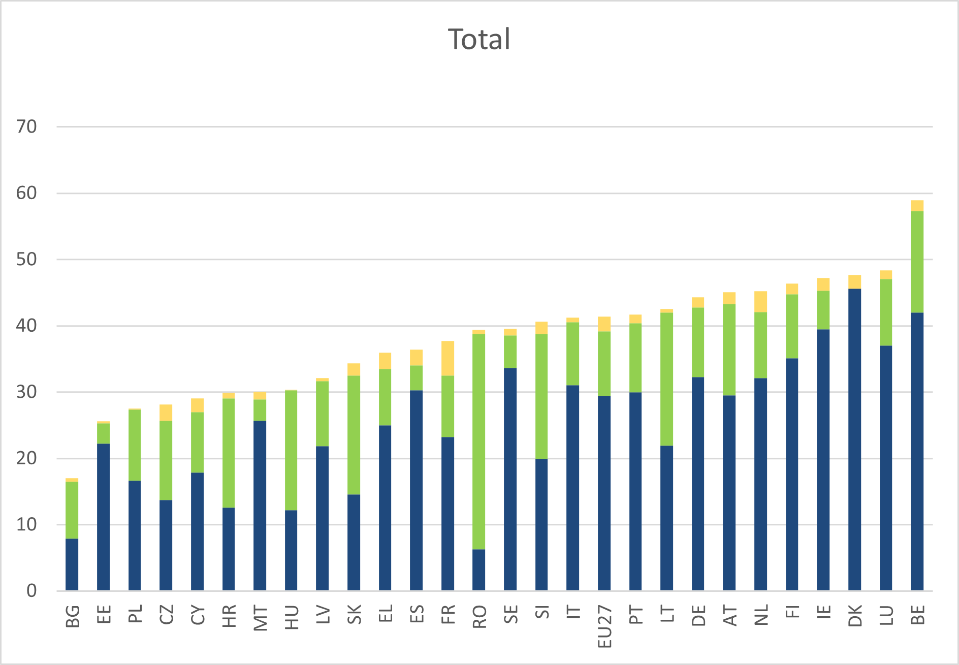


Source: JRC calculations based on EUROMOD, version I6.0+.