General labour market conditions in the EU and its Member States
Annex 1.1: further analysis and selected graphs
Box 1.3: The determinants of the job separation rate
The job separation rate is a key parameter influencing inflows into unemployment.It determines the likelihood of job loss, and along with outflows from unemployment, the overall unemployment rate. An increase in the job separation rate shifts the Beveridge curve leftward in the unemployment-vacancy space, an effect similar to an improvement in matching efficiency. Additionally, it influences the value of keeping vacancies open versus filling them immediately, thereby affecting labour demand.
There has been a persistent decline in the job separation rate.Except for cyclical spikes, the inflow rate into unemployment has been trending downward (see Graph 1.14 in the text). Transition rate into unemployment in the US have also been trending downwards and are currently at their lowest levels (Kudlyak et al (2020); Barlevy et al (2023). This trend has been attributed to changes in social norms regarding female employment and the increased availability of maternity leave, resulting in fewer career interruptions and a lower rate of women dropping out of the labour force and subsequently flowing back into unemployment. Additionally, the ageing of the “Baby Boom” generation, with older workers experiencing steadily lower separation rates than the average (Fujita, 2012; Barlevy et al., 2023); improved matching efficiency due to better screening by hiring firms (Pries and Rogerson, 2019); a declining trend in business volatility (Fujita, 2012) have contributed to this trend. Finally, workers may have prioritised job security over higher wage growth, opting to accept lower wage growth in exchange for retaining their employment.
For the EU, there is a long-run relationship linking the job separation rate to labour shortages, the ageing of the workforce, and the matching efficiency.Econometric methods allow to estimate the long-run relationship (so-called cointegration) between variables of interest whose statistical properties (mean, variance, and autocorrelation) are changing over time . For our analysis we consider the following variables: labour shortages, proxied by the factor limiting production; the employment aged 55-64 over the employment aged 25-54; the matching efficiency obtained from an estimate of the matching function. The existence of a long-run relationship is confirmed by cointegration tests that do not require any assumption on the exogeneity of the regressions (see table). The results suggest that a one percentage point increase in the share of older workers relative to the prime age group reduces the job separation rate by 50 %. Additionally, a one percentage point increase in labour shortages reduces the job separation rate by 0.2 %. This confirms that, when faced with labour shortages, companies are more cautious about dismissing their workforce.
Long-run determinants of the job separation rate (cointegration equation)
| Full Modified Least Squares | Dynamic Least Squares | Canonical Cointegrating Regression | |
|---|---|---|---|
| Labour shortages | -0.15 *** (0.02) |
-0.16 *** (0.02) |
-0.15 *** (0.02) |
| Share of employment 55-64 over share of employment 25-54 | -0.51 *** (0.03) |
-0.62 *** (0.03) |
-0.49 *** (0.03) |
| Matching efficiency | -0.15 ** (0.07) |
-0.13 (0.14) |
-0.19 *** (0.08) |
| R-squared (adjusted) | 0.82 | 0.89 | 0.80 |
| Phillips-Ouliaris cointegration test. H0: series are not cointegrated | p-value 0.0022 |
p-value 0.0022 |
p-value 0.0022 |
- Related note aThe reason is that when firms face smaller shocks it is less likely that the profitability of a job match will fall below a threshold that would lead to dismissal, resulting in lower job destruction rate (Fujita, 2023).
- Related note bThis means that the time series does not revert to a long-term mean, i.e. shocks tend to be highly persistent. In this case, the series are said to be non-stationary) .
- Related note cUnit root tests (ADF; PP and KPSS) confirms that all series are non-stationary. Matching efficiency is non-stationary when accounting for a break, which is identified in the first quarter of 2011. The matching efficiency is obtained from a Cobb-Douglas matching function defined over the total number of unemployed and vacancies
Box 1.4: The determinants of firms’ recent tendency to engage in labour hoarding
Both demand and supply factors have incentivised firms to retain more workers than needed for production during the economic slowdown, a practice known as labour hoarding.Labour market tightness (the ratio between vacancies and unemployment) and profit margins (the ratio between the GDP deflator and unit labour costs) drive changes in labour demand over the cycle. An increase in labour demand raises labour market tightness and reduces firms tendency to retain more workers than needed. Similarly, rising profit margins during a recovery spur employment. Labour shortages, which are likely to be also driven by demographic change (see also Chapter 3), and supply chain pressures capture supply-side constraints. Labour shortages induce firms to retain their workforce, while supply chain disruptions push costs up, encouraging a shift to less energy-intensive, more labour-intensive industries. Finally, better matching of vacant jobs with job seekers (matching efficiency), improves employment prospects, making employers more cautious about layoffs (1). The findings of the regression (Table 1) suggest that labour hoarding increases with intensified supply constraints but weakens with tight labour market conditions and higher profit margins (2).
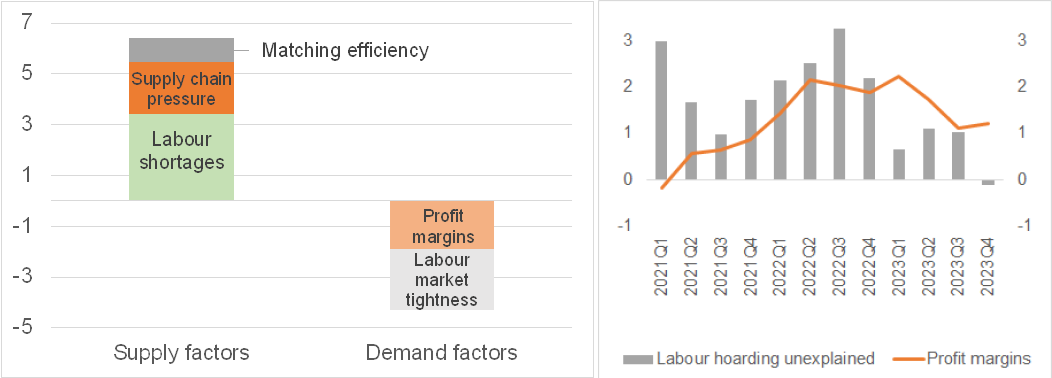
Labour shortages and labour market tightness are the main drivers of labour hoarding.To ensure consistency across variables with different variability, shocks are quantified based on the average variability of each variable, typically measured by the standard deviation. Among the supply factors, labour shortages appear to be the most important driver of labour hoarding. Labour hoarding rises by 3.5 pps in response to a shock to labour shortages (Graph 1, left panel). This figure rises to 5.5 pps in response to a supply chain disruption shock and reaches almost 6.5 pps when the effect of a shock to matching efficiency is included. Conversely, an increase in demand reduces labour hoarding by about 4 pps. Labour market tightness seems to be a more important demand-side factor than profit margins.
Graph 1: Change in labour hoarding in response to demand and supply factors and role of profit margins
Note:
The response is computed multiplying the standard deviation of each variable over the period 2020Q1-2023Q4 by the coefficients in column 8 of Table 1. In the right panel, profit margins are relative to the historical average.
Table 1: Determinants of labour hoarding in the EU over different sample periods

Note:
t-student in brackets; Robust standard errors. The matching efficiency is the residual of an estimate of a matching function obtained with OLS regression of the job finding rate on the labour market tightness for the pre-pandemic period. All regressions exclude the second quarter of 2020.
Box 1.5: Measuring labour market mismatch and reallocation
The mismatch index is based on Sahin et al. (2014).The index measures the hires that are lost due to misallocation of job seekers. It is obtained comparing the actual allocation of unemployed workers to an ideal one where job seekers can be allocated to different sectors without impediments, given the observed distribution of productivity, matching efficiency, and vacancies across sectors. This is obtained comparing the actual number of hires (h) to an ideal number of hires (h*) obtained assuming that workers can move freely between different sectors. In this ideal economy, job seekers are employed in industries with higher vacancies and matching efficiency, i.e. they search in the “right sectors”. The optimal allocation implies that the probability to find a job is equal across sectors and determines the optimal number of hires. The mismatch index is defined as the fractions of hires lost due to misallocation of actual hires relative to the optimal ones,
where 𝜑𝑖 is the matching efficiency of each industry i; 𝜑𝑖 is an average matching efficiency weighted with the share of vacancies: and the share of unemployed stemming from each sector; 𝛼 is the elasticity of the matching function and represents by how much the probability of finding a job changes when labour market tightness (labour demand) increases. The mismatch is lower the more job seekers and vacancies are aligned, for example when many are searching for a job in a sector with many vacancies. Conversely, if the number of unemployed increases in industries with a low number of vacancies, the index will increase, indicating an inefficient distribution of labour supply across industries. The index equals zero when there is no mismatch and one when there is maximal mismatch. It is also invariant to aggregate shocks that change the total number of vacancies and unemployed without altering their distribution. It is also increasing in the level of disaggregation, which implies that statements regarding mismatch should be qualified with respect to the degree of sectoral disaggregation that is used. The index has been updated for the post-pandemic period by Consolo et al (2022) and individual countries (the UK, Patterson et al 2013; Germany, Bauer, 2013; France, Chalom et al, 2018; Austria, Boheim et al, 2022.
The indicator is obtained combining different datasets.Building the indicator requires a detailed breakdown of unemployment and vacancies by sector. As concerns vacancies, the EU aggregate was obtained aggregating data by country and, when necessary, making data interpolations and splines in case of missing observations. . These data, available at quarterly frequencies, were transformed in annual by averaging to match the frequency of the unemployed data by sector of origin. The indicator requires a measure of matching efficiency by sector which cannot be computed for the EU due to the lack of data of job finding rates at sectoral levels. For this reason, the chart in the chapter shows the Sahin et al baseline index obtained in absence of heterogeneity with respect to matching efficiency. The elasticity of the matching function is set to 0.3. Higher values of α imply higher mismatch but would not its evolution over time. With the available data it was only possible to match the distribution of vacancies with that of sectors only for eleven sectors; this has implications on the level of the index but probably less on its evolution over time.
Excess job reallocation is defined as the sum of gross job creation and absolute gross job destruction minus the absolute value of the net employment change.The excess job reallocation therefore indicates the amount of job movements above what is required to accommodate the observed net employment change. Similarly to Barrero et al (2021), the excess job reallocation rate at quarter t is
Where gity is the yearly growth rate for sector I obtained adding the half yearly growth rates of the previous and of the following two quarters: ; is the share of total employment in sector i and quarter t. Growth rates are computed as half yearly employment changes as a percentage of the average employment between the initial and the final quarter: . Calculation is based on a disaggregation of employment in 86 industries. Quarterly data are subsequently averaged to get annual figures.
Graph 1.19: Change in unemployment rate during different periods (pps relative to the start of each period)

Note:
Evolution of the unemployment rate (une_rt_m) for different age groups from the lowest unemployment rate level of each period. In grey months of recession (i.e. two consecutive quarters of negative GDP growth quarter-over-quarter). M1: January; M2: February; M3: March; M4: April; M5: May; M7 July; M9: September.
Source:
Own calculations based on Eurostat, Labour Force Survey (LFS).
Graph 1.20: Job vacancy rate by country

Source:
Eurostat, job vacancy statistics.
Graph 1.21: Macroeconomic skill mismatch indicator

Note:
The macroeconomic skill mismatch indicator measures the relative dispersion of employment rates by educational levels. Q1: First quarter.
Source:
Own computations.
Graph 1.22: Contribution to economic growth in 2023 of hourly productivity, average hours worked and employment

Source:
Eurostat, National accounts.
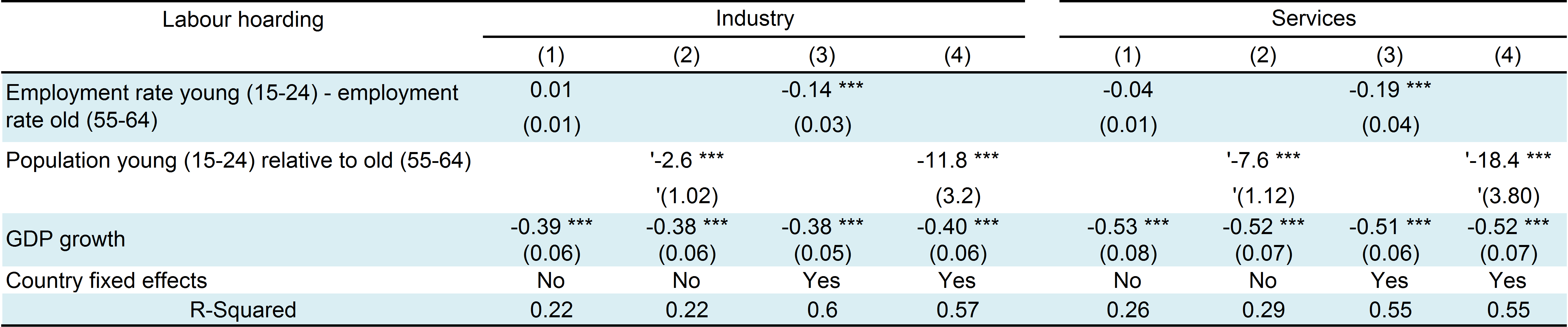
Table 1.3: Determinants of labour hoarding (panel regression)
Note:
Panel corrected robust standard error; Feasible Generalised Least Squares to control for cross-section heteroscedasticity. Sample period: 2013Q1-2024Q1; *** significant at 1%.